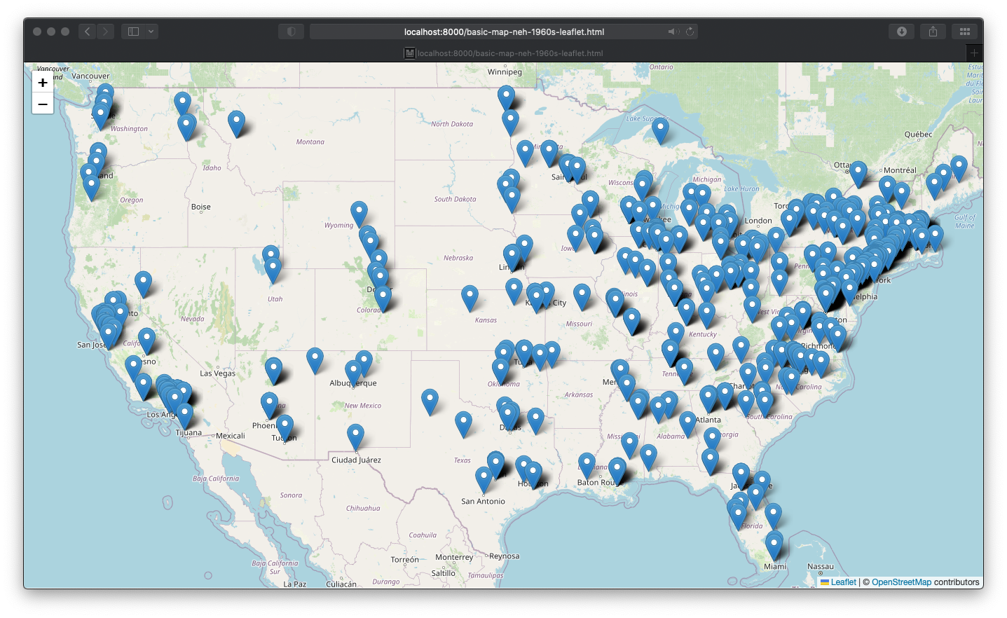
This is a post in my occasional humanities data curation series, which outlines humanities data curation activities using publicly-available data on grants and awards made by the National Endowment for the Humanities (NEH). A subset of the series focuses on mapping the data and creating geospatial data visualizations.
For reference, here are the other essays in the series:
-
Metadata: Origins and Metaphors (10 September 2024)
-
Encoding Reparative Description: Preliminary Thoughts (17 September 2023)
-
Find and replace data in the shell (11 September 2022)
-
Wrangling Humanities Data: An Interactive Map of NEH Awards (17 July 2022)
-
Wrangling Humanities Data: Using Regex to Clean a CSV (27 February 2021)
-
Wrangling Humanities Data: Exploratory Maps of NEH Awards by State (22 January 2021)
-
Wrangling Humanities Data: Cleaning and Transforming Data (19 January 2021)
-
Wrangling Humanities Data: Finding and Describing Data (20 December 2020)
This installment uses the geospatial dataset previously created and describes how to display the data in an interactive map on the web. As in the previous post, you can also download a version of this post from the GitHub repository along with all of the data discussed here. File references discussed below are included in the same neh-grant-data-project repository.
Mapping the data on an interactive, web-based map
Although my previous essays have explored various data-related topics, this post continues a theme of mapping humanities data. Previous installments walked through the process of preserving, transforming, and visualizing this data, which is a list of grants awarded by the NEH during the 1960s (the agency’s first five years). This post demonstrates how to create interactive, web-friendly maps more familiar to everyday users. The goal is to plot the grant information from the 1960s on a map background that allows zooming in and out, repositioning, and the option to click on each point to get information about the referenced grant.
Mapping the geojson
Rather than building the map from scratch (as previously), this demonstration uses widely used, open, and pre-existing code libraries to generate the map with the desired features. The primary tool is Leaflet.js, a javascript library that will knit together the map tiles and the grant data.
Leaflet provides a library of tools, written in javascript, that help to display geospatial information via a web browser. By combining this library, which builds on common frameworks and code approaches to web publishing, with the geospatial grant data, we can create, display, and share the map. The elements that power the map include:
- an HTML file that will pull in leaflet and create the basic page framework for the map
- a CSS file to style and modify the display of the map
- a javascript file that will use the leaflet tools to extract and load the geojson data
A similar process is outlined in a clear and approachable way by Kim Pham in “Web Mapping with Python and Leaflet,” Programming Historian 6 (2017), doi:10.46430/phen0070. Pham’s tutorial starts by setting up all of the map elements in one file (with a different dataset), then splits them out into three files as below. If you want to see how this would look in one file, refer to the above tutorial.
Because the html and css elements of this step are the shortest, we will go through those first. Below is a walkthrough description of each file.
HTML
The first file is an html file (basic-map-neh-1960s-leaflet.html).
In the <head> section, this file calls the necessary javascript and css files that are required for operating the Leaflet library. The header also pulls in a custom css file for our map (see the next file walkthrough).
In the <body> section, the html includes only one empty div with an id="map" attribute. This tag is all that we need to provide the page information that leaflet can hook the full map on.
Finally, just before the closing </html> tag, the file references the javascript file that we will use to create the map (see the subsequent file walkthrough).
<!DOCTYPE html>
<head>
    <link rel="stylesheet" href="https://unpkg.com/leaflet@1.8.0/dist/leaflet.css" integrity="sha512-hoalWLoI8r4UszCkZ5kL8vayOGVae1oxXe/2A4AO6J9+580uKHDO3JdHb7NzwwzK5xr/Fs0W40kiNHxM9vyTtQ==" crossorigin="" />
    <script src="https://unpkg.com/leaflet@1.8.0/dist/leaflet.js" integrity="sha512-BB3hKbKWOc9Ez/TAwyWxNXeoV9c1v6FIeYiBieIWkpLjauysF18NzgR1MBNBXf8/KABdlkX68nAhlwcDFLGPCQ==" crossorigin=""></script>
    <script src="https://code.jquery.com/jquery-2.1.4.min.js"></script>

    <link rel="stylesheet" href="basic-map-neh-1960s-leaflet.css" />

</head>
<body>

    <div id="map"></div>

</body>
    <script src="basic-map-neh-1960s-leaflet.js"></script>
</html>
CSS
Next is a short css file (basic-map-neh-1960s-leaflet.css).
This file provides styling information to the browser about how to display the map. Most important is the information for the map id, which provides
instructions to the browser about where to display the leaflet map.
body {
    margin: 0;
    padding: 0;
}
#map {
    position: absolute;
    top: 0;
    bottom: 0;
    width: 100%;
    height: 750px;
}
Javascript for leaflet
The file that pulls this all together is the javascript that calls
the leaflet functions to create the map, load the grant data, and creates individual markers for each grant point (basic-map-neh-1960s-leaflet.js)
The file opens by calling a function via window.onload. This means that each time the window is loaded (or reloaded), the browser will execute
the instructions to draw (or redraw) the map.
Next, we create a basemap variable (var basemap), which provides information about the underlying map layer. In this case, we draw the tiles from the Open Street Map project and provide attribution.
Then, the $.getJSON command loads the geojson data (created previously).
Using leaflet’s functions (they are recognizably prepended with L.), the file
gives instructison for parsing each geojson element into points. The majority of this section is a series of filters that provide information
for displaying the text (e.g., how to display the integers as US dollars) or correcting missing information (such as unlisted Institution fields). At the end of this block, in the layer.bindPopup statement, a formatted
string creates the text of the popup for each grant on the map.
Finally, leaflet is instructed to draw the map. The view is set (zoom level and the latitude and longitude to center the view). And, the basemap and geojson are added as layers to the interactive map.
The next section explains how to use python locally to view (serve) these files and explore the interactive map as it could appear if published to the web.
window.onload = function () {
var basemap = L.tileLayer('http://{s}.tile.osm.org/{z}/{x}/{y}.png', {
attribution: '© <a href="http://osm.org/copyright">OpenStreetMap</a> contributors'
});
// retrieve the geojson data
$.getJSON("neh_1960s_grants.geojson", function(data) {
// set popups for each point
var geojson = L.geoJson(data, {
onEachFeature: function (feature, layer) {
// set content formatting to format and correct missing information for popups
if ( feature.properties.Institution == null ) {
feature.properties.Institution = 'an unaffiliated, independent scholar'
}
if ( feature.properties.Participants == null ) {
feature.properties.Participants = 'unlisted'
}
if ( feature.properties.ProjectTitle == null ) {
feature.properties.ProjectTitle = 'unlisted'
}
let dollarUS = Intl.NumberFormat('en-US', {
style: 'currency',
currency: 'USD',
})
// create the popups
layer.bindPopup(
`<p>In ${ feature.properties.YearAwarded }, ${ feature.properties.Institution } (in ${ feature.properties.InstCity }, ${ feature.properties.InstState }) was awarded ${ dollarUS.format(feature.properties.AwardOutright) } for <a href="https://securegrants.neh.gov/publicquery/main.aspx?f=1&gn=${ feature.properties.AppNumber }">NEH project number ${ feature.properties.AppNumber }</a>.<br /><br /><strong>Project Title:</strong> ${ feature.properties.ProjectTitle }<br /><strong>Project participants:</strong> ${ feature.properties.Participants }<br /><strong>NEH Program:</strong> ${ feature.properties.Program }<br /><strong>NEH Division:</strong> ${ feature.properties.Division }</p>`
);
}
});
// set up the map, set viewport
var map = L.map('map')
.setView([37.90, -94.66], 4); //continental US view
basemap.addTo(map);
geojson.addTo(map);
});
};
Getting it up and running
After files are created, we can use the python HTTP server to display the files locally and see how they may display on the live web. For this, use python3 http.server module. (Note: this should only be used locally for testing, not in a production environment.)
To display (and “run” the files) the files with python, open a command shell, navigate to the location where the files are stored, then run:
python -m SimpleHTTPServer or in python3 python3 -m http.server.
You can specify a server port for these if you like, or you can use the default. When the server starts, you will see something like this displayed in the shell:
Serving HTTP on 0.0.0.0 port 8000 ....
Note the port number. Now, open a web browser. In the browser’s location bar, use the port number (rather than a URL) to display the local server. For example, if as above the port is 800, you would request the following address in the browser:
localhost:8000/ or 127.0.0.1:8000
If the files are working correctly, you should see something like a map dotted with blue markers representing the grant data.


Comments